CALIBRATED CONFIDENCE INTERVALS FOR INTENSITIES OF A TWO STAGE OPEN QUEUEING NETWORK WITH FEEDBACK

GEDAM V.K.; PATHARE S.B.

CALIBRATED CONFIDENCE INTERVALS FOR INTENSITIES OF A TWO STAGE OPEN QUEUEING NETWORK WITH FEEDBACK

GEDAM V.K.¹, PATHARE S.B.²*
¹Department of Statistics, University of Pune- 411007, MS, India.
²Indira College of Commerce and Science, Pune- 411033, MS, India.
* Corresponding Author : sureshpathare23@gmail.com

Received : 02-08-2013 Accepted : 22-08-2013 Published : 07-09-2013
Volume : 4 Issue : 1 Pages : 151 - 161
J Stat Math 4.1 (2013):151-161

Cite - MLA : GEDAM V.K. and PATHARE S.B. "CALIBRATED CONFIDENCE INTERVALS FOR INTENSITIES OF A TWO STAGE OPEN QUEUEING NETWORK WITH FEEDBACK." Journal of Statistics and Mathematics 4.1 (2013):151-161.

Cite - APA : GEDAM V.K., PATHARE S.B. (2013). CALIBRATED CONFIDENCE INTERVALS FOR INTENSITIES OF A TWO STAGE OPEN QUEUEING NETWORK WITH FEEDBACK. Journal of Statistics and Mathematics, 4 (1), 151-161.

Cite - Chicago : GEDAM V.K. and PATHARE S.B. "CALIBRATED CONFIDENCE INTERVALS FOR INTENSITIES OF A TWO STAGE OPEN QUEUEING NETWORK WITH FEEDBACK." Journal of Statistics and Mathematics 4, no. 1 (2013):151-161.

Copyright : © 2013, GEDAM V.K. and PATHARE S.B., Published by Bioinfo Publications. This is an open-access article distributed under the terms of the Creative Commons Attribution License, which permits unrestricted use, distribution and reproduction in any medium, provided the original author and source are credited.

Abstract

The aim of this paper is to provide an approximate 100(1-Î±)% calibrated CAN, Exact t, Standard Bootstrap, Bootstrap-t, Variance-stabilized Bootstrap-t, Bayesian Bootstrap, Percentile Bootstrap and Bias-corrected and accelerated bootstrap confidence intervals for intensity parameters of a two stage open queueing network with feedback with distribution-free interval and service times. Numerical simulation study is conducted to demonstrate performances of the confidence intervals by using calibration technique. We consider a measure, named relative coverage, to evaluate performances of the said intervals.

Keywords

Calibration, calibrated confidence intervals, Coverage percentage, Relative coverage.

Introduction

Calibration technique is used for improving the coverage accuracy of any system of approximate confidence intervals. The general theory of calibration is reviewed in Efron and Tibshirani [6] , following ideas of Loh [16] , Beran [1] , Hall [11] and Hall and Martin [12] . The bootstrap calibration technique was introduced by Loh [16,17] . The idea of the bootstrap calibration is to first use bootstrap to estimate the true coverage of confidence intervals and the intervals is then adjusted by comparing with the target nominal level. As we aware that in literature, no work regarding the calibration technique in queueing networks is found. So it is tempting to use calibration technique to construct new confidence intervals called calibrated confidence interval for intensity parameters of a two stage open queueing network whose true coverage probabilities come closer to desired value.
Consider a network model of a computer system with feedback in which a job may return to previously visited nodes. The system consists of two nodes CPU node and I/O node with respective service rates µ₁ and µ₂. The external arrival rate is λ. After service completion at CPU node, the job proceeds to the I/O node with probability p₁, and departs from the system with probability p₀ where p₀ = 1-p₁. Jobs leaving the I/O node are always feed back to the CPU node [Fig-1] . The successive service time at both nodes are assumed to be mutually independent and independent of the state of the system.
The traffic intensities at the CPU node and I/O node are respectively given by

$\rho _{1}=\frac{\lambda }{p_{0}\: \mu _{1}},\rho _{2}=\frac{p_{1}\lambda }{p_{0}\: \mu _{2}}$ (1)

where ρ₁ and ρ₂ can be interpreted as expected number of arrivals per mean service time. The condition for stability of the system is both ρ₁ and ρ₂ are less than unity.
Burke [2] has shown that the output of an M/M/1 queue is also Poisson with rate λ. Jackson [14] showed that the product form solution also applies to open network of Markovian queues with feedback, also Jackson’s theorem states that each node behaves like an independent queue. Disney [3] introduces basic properties of queueing networks. Thiruvaiyaru, Basawa and Bhat [23] established maximum likelihood estimators of the parameters of an open Jackson network. Thiruvaiyaru and Basawa [22] considered the problem of estimation for the parameters in a Jackson’s type queueing network.
Efron [7-9] the greatest statistician in the field of nonparametric resampling approach, originally developed and proposed the bootstrap, which is a resampling technique that can be effectively applied to estimate the sampling distribution of any statistic. For necessary background on bootstrap technique, we refer to Efron and Gong [4] , Efron and Tibshirani [5] , Guntur [10] , Mooney and Duval [19] , Young [24] , Rubin [21] , Miller [18] . Ke and Chu [15] constructed various confidence intervals for intensity parameter of a queueing system.

Nonparametric Statistical Inference of Intensities

Let (X_i, Y_i, i = 1,2) be nonnegative random variables representing the inter-arrival and service times of CPU and I/O node respectively. Once a job complete CPU node burst, it will proceed to I/O node for further service with probability p₁ and departs from the system with probability p₀ where p₀ = 1- p₁. Then the intensities are defined as follows:

$\rho _{1}=\frac{p_{0}\: \mu _{Y_{1}}}{\mu _{X_{1}}}\: and\: \rho _{2}=\frac{p_{0}\: \mu _{Y_{2}}}{p_{0}\: \mu _{X_{2}}}$

Where $\mu _{X_{1}}\: and\: \mu _{X_{2}}$ denote the mean inter-arrival times and $\mu _{Y_{1}}\: and\: \mu _{Y_{2}}$ denote the mean service times of CPU node and I/O node respectively.
Assume that (X_1j, p₀ Y_1j, j= 1,2...n) is a random sample drawn from (X₁, Y₁) and (p₁ X_2j, p₀ Y_2j, j= 1,2...n) is a random sample drawn from(X₂, Y₂). Define $(\bar{X_{i}},\bar{Y_{i}},i=1,2)$ to be the sample means of (X_i, Y_i, i= 1,2) respectively. Thus according to the Strong Law of Large Numbers [20] ; we know that $(\bar{X_{i}},\bar{Y_{i}},i=1,2)$ are strongly consistent estimator of $(\mu _{x_{i}},\mu _{y_{i}},i=1,2)$ respectively. Thus strongly consistent estimators of intensities are given by $\hat{\rho _{i}}=\frac{\bar{Y_{i}}}{\bar{X_{i}}},\: \: i=1,2$ . The true distributions of (X_i, Y_i, i= 1,2) are not often known in practice so the exact distributions of $\hat{\rho _{i}}$ , i= 1,2 cannot be derived. But under the assumption that X_i and Y_i being independent, the asymptotical distributions of $\hat{\rho _{i}}$ . i= 1,2 can be developed as the following procedures. By Central Limit Theorem and Slutsky’s theorem [13] , we have

$\sqrt{n}\: (\hat{\rho _{i}}-\rho _{i})\overset{D}{\rightarrow}N\: (0,\sigma _{i}^{2}),i=1,2.$

Where

$\sigma _{i}^{2}=(\mu _{X_{1}}^{2}\: \sigma _{Y_{1}}^{2}+p_{0}^{2}\: \mu _{Y_{1}}^{2}\: \sigma _{X_{1}}^{2})/\mu _{X_{1}}^{4}\: and\: \sigma _{2}^{2}=(p_{1}^{2}\: \mu _{X_{2}}^{2}\: \sigma _{Y_{2}}^{2}+p_{0}^{2}\: \mu _{Y_{2}}^{2}\sigma _{X_{2}}^{2})/(p_{1}^{2}\: \mu _{X_{2}}^{4})$

Also, $\overset{D}{\rightarrow}$ denotes convergence in distribution.
Now set

$\hat{\sigma }_{1}^{2}=\bar{X}_{1}^{2}\: S_{Y_{1}}^{2}+p_{0}^{2}\: \bar{Y}_{1}^{2}\: S_{X_{1}}^{2}/\bar{X}_{1}^{4}\: and\: \hat{\sigma }_{2}^{2}=p_{1}^{2}\: \bar{X}_{2}^{2}\: S_{Y_{2}}^{2}+p_{0}^{2}\: \bar{Y}_{2}^{2}\: S_{X_{2}}^{2}/p_{1}^{2}\: \bar{X}_{2}^{4}$

where

$S_{X_{1}}^{2}=\frac{1}{n}\sum_{j=1}^{n}(X_{1j}-\bar{X}_{1})^{2},S_{X_{2}}^{2}=\frac{1}{n}\sum_{j=1}^{n}(p_{1}\: X_{2j}-\bar{X}_{2})^{2},S_{Y_{1}}^{2}=\frac{1}{n}\sum_{j=1}^{n}(p_{0}\: Y_{1j}-\bar{Y}_{1})^{2}\: and\: S_{Y_{2}}^{2}=\frac{1}{n}\sum_{j=1}^{n}(p_{0}\: Y_{2j}-\bar{Y}_{2})^{2}$

Then $\hat{\sigma }_{i}^{2}$ , i= 1,2 is strongly consistent estimator of $\hat{\sigma }_{i}^{2}$ , i= 1,2. Again applying the Slutsky’s theorem we have

$\frac{\sqrt{n}(\hat{\rho }_{i}-\rho _{i})}{\hat{\sigma }_{i}}\overset{D}{\rightarrow}N(0,1),i=1,2.$

Thus $\hat{\rho }_{i}$ , i= 1,2 is strongly consistent and asymptotically normal (CAN) estimator with approximate variances $\hat{\sigma }_{i}^{2}/n$ , i= 1,2.

Calibration Technique

Let a confidence limit $\hat{\rho }_{i}$ [ α ] is supposed to have probability α of covering the true value ρ_i, that is, $P_{F_{i}}\left \{ \rho _{i}\leq \hat{\rho _{i}}(\alpha ) \right \}=\alpha ,i=1,2$ where F_i is unknown continuous probability distribution. Thus ρ_i is supposed to be less than $\hat{\rho _{i}}$ [0. 95], 95% of the time and $\hat{\rho _{i}}$ [0. 05], 5% of the time. For an approximate confidence limit there is true probability β_i that ρ_i is less than $\hat{\rho _{i}}$ [ α ] say, $\beta _{i}(\alpha )=P_{F_{i}}\left \{ \rho _{i}\leq \hat{\rho _{i}}(\alpha ) \right \}$ .
The actual coverage of a confidence procedure is rarely equal to the desired coverage and often it is substantially different. If we knew the function β_i(α) then we could calibrate an approximate confidence interval to give exact coverage. Suppose we know that β_i(0.03)=0.05 and β_i(0.94)=0.95. Then instead of ( $\hat{\rho _{i}}$ [0. 05], $\hat{\rho _{i}}$ [0. 95]) we would use ( $\hat{\rho _{i}}$ [0. 03], $\hat{\rho _{i}}$ [0. 94]) to get a central 90% interval with correct coverage probabilities.
In practice we usually don’t know the calibration function β_i(α). However we can use the bootstrap to estimate β_i(α). The bootstrap estimate of β_i(α) is $\hat{\beta _{i}}(\alpha )=P_{\hat{F}_{i}}\left \{ \hat{\rho _{i}}\leq \hat{\rho _{i}}(\alpha )^{\ast } \right \}$ where $\hat{F}_{i}$ and $\hat{\rho }_{i}$ are fixed, nonrandom quantities and $\hat{\rho }_{i}$ [ α ]^* is the α^th confidence limit based on bootstrap dataset from $\hat{F}_{i}$ . The estimate $\hat{\beta }_{i}\: (\alpha )$ is obtained by taking B bootstrap data sets and seeing what proportion of them have $\hat{\rho }_{i}\leq \hat{\rho }_{i}$ [ α ]^*.

CAN Calibrated Confidence Interval

Using the CAN estimators $\hat{\rho }_{i}$ , i= 1,2 and its associated approximate variances $\hat{\sigma }_{i}^{2}/n$ , i = 1,2, we construct calibrated confidence intervals for intensities ρ_i, i= 1,2 of a two stage open queueing network with feedback. Let Z_α be the upper α^th quantile of the standard normal distribution.
Compute $\hat{\beta }(\alpha )=P\left \{ \rho _{i}\leq (\hat{\rho }_{i}-Z_{a/2}\: \hat{\sigma }_{i}/\sqrt{n}) \right \}$ and $\hat{\beta }(1-\alpha )=P\left \{ \rho _{i}\leq (\hat{\rho }_{i}+Z_{a/2}\: \hat{\sigma }_{i}/\sqrt{n}) \right \}$
By the asymptotic distribution of $\frac{\sqrt{n}\: (\hat{\rho }_{i}-\rho _{i})}{\hat{\sigma }_{i}},i=1,2$ an approximate 100 (1 - α) % calibrated confidence intervals for ρ_i, i= 1,2 are given as

$\left ( \hat{\rho }_{i}\: '-z_{\hat{\beta }(\alpha )/2}\: \hat{\sigma }_{i}\: '/\sqrt{n},\: \hat{\rho }_{i}\: '+z_{(1-\hat{\beta }(1-\alpha ))/2}\: \hat{\sigma }_{i}\: '/\sqrt{n} \right )i=1,2$ (2)

Exact- t Calibrated Confidence Interval

Let tα be the upper αth quantile of the Student’s t-distribution.
Compute $\hat{\beta }(\alpha )=P\left \{ \rho _{i}\leq (\hat{\rho }_{i}-t_{(n-1),\: a/2}\: \hat{\sigma }_{i}/\sqrt{n}) \right \}$ and $\hat{\beta }(1-\alpha )=P\left \{ \rho _{i}\leq (\hat{\rho }_{i}+t_{(n-1),\: a/2}\: \hat{\sigma }_{i}/\sqrt{n}) \right \}$
Then an approximate 100(1-α)% exact-t calibrated confidence intervals for ρ_i, i= 1,2 are given as
$\left ( \hat{\rho }_{i}\: '-t_{(n-1),\: \hat{\beta }(\alpha )/2}\: \hat{\sigma }_{i}\: '/\sqrt{n},\: \hat{\rho }_{i}\: '+t_{(n-1),\: (1-\hat{\beta }(1-\alpha ))/2}\: \hat{\sigma }_{i}\: '/\sqrt{n} \right )i=1,2$ (3)

Standard Bootstrap Calibrated Confidence Interval

Using bootstrap procedure, a simple random samples
$(X_{ij}^{\ast },\: p_{0}\: Y_{ij}^{\ast },\: i=1;j=1,2,....n)$ and $(p_{1}\: X_{ij}^{\ast },\: p_{0}\: Y_{ij}^{\ast },\: i=2;j=1,2,....n)$
are taken from the empirical distribution functions of (X_ij, p₀ Y_ij, i=1; j= 1,2...n) and (p₁ X_ij, p₀ Y_ij, i=2; j = 1,2...n). Bootstrap estimate of ρ_i, i= 1,2 is calculated as $\hat{\rho }_{i}^{\ast }=\frac{\bar{y}_{i}^{\ast }}{\bar{x}_{i}^{\ast }},\: i=1,2$ . The above resampling process is repeated N times and $\hat{\rho }_{i1}^{\ast },\: \hat{\rho }_{i2}^{\ast },\: ...\: ,\hat{\rho }_{iN}^{\ast },\: i=1,2$ are computed from the bootstrap re-samples. Averaging the N bootstrap estimates we get bootstrap estimate of ρ_i, i= 1,2 as
$\hat{\rho }_{N}\: (i)=\frac{1}{N}\sum_{j=1}^{N}\: \hat{\rho }_{ij}^{\ast },\: i=1,2$ and standard deviation of $\hat{\rho }_{i}$ , i= 1,2 is

$sd\: (\hat{\rho }_{N}\: (i))=\left \{ \frac{1}{N-1}\sum_{j=1}^{N}(\hat{\rho }_{ij}^{\ast }-\hat{\rho }_{N}\: (i))^{2} \right \}^{1/2},i=1,2.$

Then by central limit theorem, the distribution of $\hat{\rho }_{i}$ , i= 1,2 is approximately normal. Compute

$\hat{\beta }(\alpha )=P\left \{ \rho _{i}\leq (\hat{\rho }_{i}-z_{a/2}\: sd\: (\hat{\rho }_{N}(i))) \right \}$ and $\hat{\beta }(1-\alpha )=P\left \{ \rho _{i}\leq (\hat{\rho }_{i}+z_{a/2}\: sd\: (\hat{\rho }_{N}(i))) \right \}$

Then 100(1-α)% SB calibrated confidence interval for ρ_i as,

$\left ( \hat{\rho }_{i}\: '-z_{\hat{\beta }(\alpha )/2}\: sd\: '(\hat{\rho }_{N}(i)),\: \hat{\rho }_{i}\: '+z_{(1-\hat{\beta }(1-\alpha ))/2}\: sd\: '(\hat{\rho }_{N}(i)) \right )i=1,2$ (4)

Bootstrap-t Calibrated Confidence Interval

Consider N bootstrap estimates $\hat{\rho }_{i1}^{\ast },\: \hat{\rho }_{i2}^{\ast },\: ...\: ,\: \hat{\rho }_{iN}^{\ast },i=1,2$ computed from the bootstrap resample. We compute
$Z_{ij}^{\ast }=\frac{(\hat{\rho }_{ij}^{\ast }-\: \hat{\rho }_{N}(i))}{\mathrm{sd}\: (\hat{\rho }_{N}(i))},i=1,2,j=1,2\: ....\: N$ and $Z_{ij}^{\ast },\: i=1,2\: .\: j=1,2\: ....\: N$
follow an approximate t distribution. Also compute

$\hat{\beta }(\alpha )=P\left \{ \rho _{i}\leq (\hat{\rho }_{i}-t_{a/2}\: sd\: (\hat{\rho }_{N}(i))) \right \}$ and $\hat{\beta }(1-\alpha )=P\left \{ \rho _{i}\leq (\hat{\rho }_{i}+t_{a/2}\: sd\: (\hat{\rho }_{N}(i))) \right \}$

Then 100(1-α)% Bootstrap-t calibrated confidence interval for ρ_i is

$\left ( \hat{\rho }_{i}\: '-\hat{t}_{\hat{\beta }(\alpha )/2}\: sd\: '(\hat{\rho }_{N}(i)),\: \hat{\rho }_{i}\: '+\hat{t}_{(1-\hat{\beta }(1-\alpha ))/2}\: sd\: '(\hat{\rho }_{N}(i)) \right )i=1,2$ (5)

Where $\hat{t}_{\hat{\beta }(\alpha )/2}$ and $\hat{t}_{(1-\hat{\beta }(1-\alpha ))/2}$ equals the α/2 and (1-α/2) percentile of the random sample $Z_{i1}^{\ast },Z_{i2}^{\ast },...,Z_{iN}^{\ast },i=1,2$ .

Variance-stabilized Bootstrap-t Calibrated Confidence Interval

Let $\hat{\rho }_{i}$ , i= 1,2 be a strongly consistent and asymptotically normal estimator with approximate variances $\hat{\sigma }_{i}^{2}/n,i=1,2.$ . Let $\hat{\sigma }_{i}=\phi (\hat{\rho }_{i})$
To find a transformation $f(\hat{\rho }_{i})$ such that $Var(f(\hat{\rho }_{i}))\approx$ constant, we use the first order Taylor series expansion:

$f(\hat{\rho }_{i})\approx f(\rho _{i})+(\hat{\rho }_{i}-\rho _{i})f\: '(\rho _{i})\Rightarrow (f(\hat{\rho }_{i})-f(\rho _{i}))^{2}\approx (\hat{\rho }_{i}-\rho _{i})^{2}(f'(\rho _{i}))^{2}$

Taking expectations on both sides, we get:

$Var(f(\hat{\rho }_{i}))\approx Var(\hat{\rho }_{i})(f\: '(\rho _{i}))^{2}=(\phi (\rho _{i}))^{2}(f\: '(\rho _{i}))^{2},i=1,2.$

Now consider $f(\hat{\rho }_{i})=\sqrt{n}\: \mathrm{log}\: (\phi (\hat{\rho }_{i})),i=1,2$ is the variance-stabilizing transformation. Then we have,

$V(f(\hat{\rho }_{i}))\approx \left ( \frac{\sqrt{n}}{\phi (\hat{\rho }_{i})} \right )^{2}Var(\hat{\rho }_{i})=\left ( \frac{\sqrt{n}}{\hat{\sigma }_{i}} \right )Var(\hat{\rho }_{i})=\frac{n}{\hat{\sigma }_{i}^{2}}\: \frac{\hat{\sigma }_{i}^{2}}{n}=1,i=1,2.$

Here we consider N bootstrap estimates $\hat{\rho }_{i1}^{\ast },\: \hat{\rho }_{i2}^{\ast },\: ...\: ,\: \hat{\rho }_{iN}^{\ast },i=1,2$ computed from the bootstrap resample.
We obtain $\theta _{ij}^{\ast }=(\sqrt{n}\: \mathrm{log}\: (\hat{\rho }_{ij}^{\ast })-\sqrt{n}\: \mathrm{log}\: (\hat{\rho }_{i})),i=1,2,j=1,2...N$
Also compute

$\hat{\beta }(\alpha )=P\left \{ \rho _{i}\leq e^{\mathrm{log}\: (\hat{\rho }_{i})-\frac{1}{\sqrt{n}}\: \hat{v}_{i}\: t_{1-\alpha /2}} \right \}$ and $\hat{\beta }(1-\alpha )=P\left \{ \rho _{i}\leq e^{\mathrm{log}\: (\hat{\rho }_{i})-\frac{1}{\sqrt{n}}\: \hat{v}_{i}\: t_{\alpha /2}} \right \}$

A 100(1-α)% Variance- stabilized Bootstrap-t (VST) calibrated confidence interval for ρ_i, i=1,2 is

$\left ( e^{\mathrm{log}\: (\hat{\rho }_{i})-\frac{1}{\sqrt{n}}\: \hat{v}_{i}\: t_{\hat{\beta }(\alpha )/2}},\: e^{\mathrm{log}\: (\hat{\rho }_{i})-\frac{1}{\sqrt{n}}\: \hat{v}_{i}\: t_{\hat{\beta }(1-\alpha )/2}} \right )$ (6)

Where $\hat{v}_{i}\: t_{\hat{\beta }(\alpha )/2}$ and $\hat{v}_{i}\: t_{\hat{\beta }(1-\alpha )/2}$ are α/2 and (1-α/2) percentile of the random sample $\theta _{i1}^{\ast },\theta _{i2}^{\ast },\: ...\: ,\: \theta _{iN}^{\ast },i=1,2$ .

Bayesian Bootstrap Calibrated Confidence Interval

Here each BB replication generates a posterior probability for each X_ij, i=1, j=1,2...n and p₁ X_ij, i=1, j=1,2...n. One BB replication is generated by drawing n-1 uniform (0, 1) random numbers r₁,r₂,...r_n-1, ordering them, and calculating the gaps w_j= r_(j)-r(j-1), j=1,2...n where
r₍₀₎=0 and r_(n)=1. Then w_i=(w_i1,w_i2,…,w_in), i=1,2 is the vector of probabilities attached to the inter-arrival data values (X_1j, p₁X_2j, j=1,2...n) respectively. Next considering all BB replications gives the BB distribution of the distribution of X_i and thus of any parameter of this distribution we calculate µ_xi i=1,2 (the mean of X_i), in each BB replication. Let w_ij be the probability that X_i = x_ij then we calculate $\bar{X}_{1}^{\ast \ast }=\sum_{j=1}^{n}w_{1j}\: x_{1j}$ and $\bar{X}_{2}^{\ast \ast }=p_{1}\sum_{j=1}^{n}w_{2j}\: x_{2j}$ and the distribution of the values of $\bar{X}_{i}^{\ast \ast }$ overall BB replications is the BB distribution of µ_xi.
Now generating a vector of probabilities v_i=(v_i1,v_i2,…,v_in), i=1,2 attached to the service time data values p₀Y_ij, i=1,2. j= 1,2...n in a BB replication.
We calculate $\bar{Y}_{i}^{\ast \ast }=p_{0}\sum_{j=1}^{n}v_{ij}\: y_{ij}$ for µ_xi.
Thus estimate of Intensity ρi be calculated from BB replications as
$\hat{\rho }_{i}^{\ast \ast }=\frac{\bar{Y}_{i}^{\ast \ast }}{\bar{X}_{i}^{\ast \ast }},i=1,2$ .
The above BB process can be repeated N times. The N BB estimates $\hat{\rho }_{i1}^{\ast },\hat{\rho }_{i2}^{\ast },..,\hat{\rho }_{iN}^{\ast },i=1,2$ are computed from the BB replications. Averaging the N BB estimates, we obtain that $\hat{\rho }_{BB}(i)=\frac{1}{N}\sum_{j=1}^{N}\hat{\rho }_{ij}^{\ast },i=1,2$ is the BB estimate of ρ_i, i=1,2 and the standard deviation of $\hat{\rho }_{i}$ can be estimated by

$\mathrm{sd}\: (\hat{\rho }_{BB}(i))=\left \{ \frac{1}{N-1}\: \sum_{j=1}^{N}\: (\hat{\rho }_{ij}^{\ast \ast }-\hat{\rho }_{BB}(i))^{2} \right \}^{\frac{1}{2}},i=1,2.$

Find $\hat{\beta }\: (\alpha )=P\left \{ \rho _{i}\leq (\hat{\rho }_{i}-z_{\alpha /2}\: sd\: (\hat{\rho }_{BB}\: (i))) \right \}$ and $\hat{\beta }\: (1-\alpha )=P\left \{ \rho _{i}\leq (\hat{\rho }_{i}+z_{\alpha /2}\: sd\: (\hat{\rho }_{BB}\: (i))) \right \}$
Applying the asymptotical normality of $\hat{\rho }_{i}$ , i= 1,2, The 100(1-α)% BB calibrated confidence interval for ρ_i, i= 1,2 is

$\left ( \hat{\rho }_{i}\: '-z_{\hat{\beta }\: (\alpha )\: /\: 2}\: sd\: '(\hat{\rho }_{BB}(i)),\hat{\rho }_{i}\: '+z_{(\hat{1-\beta }\: (1-\alpha ))\: /\: 2}\: sd\: '(\hat{\rho }_{BB}(i)) \right )i=1,2$ (7)

Percentile Bootstrap Calibrated Confidence Interval

Now call $\hat{\rho }_{i1}^{\ast },\hat{\rho }_{i2}^{\ast },...,\hat{\rho }_{iN}^{\ast },i=1,2$ the bootstrap distribution of $\hat{\rho }_{i}$ ,i= 1,2. Let $\hat{\rho }_{i}^{\ast }(1),\hat{\rho }_{i}^{\ast }(2),...,\hat{\rho }_{i}^{\ast }(N),i=1,2$ be the order statistics of $\hat{\rho }_{i1}^{\ast },\hat{\rho }_{i2}^{\ast },...,\hat{\rho }_{iN}^{\ast },$ i= 1,2.
Compute $\hat{\beta }(\alpha )=P\left \{ \rho _{i}\leq \hat{\rho }_{i}^{\ast }(N(\frac{\alpha }{2})) \right \}$ and $\hat{\beta }(1-\alpha )=P\left \{ \rho _{i}\leq \hat{\rho }_{i}^{\ast }(N(1-\frac{\alpha }{2})) \right \}$
Then utilizing the 100(α/2)^th and 100(1-α/2)^th percentage points of the bootstrap distribution, a 100(1-α)% PB calibrated confidence interval for ρ_i, i= 1,2 are obtained as

$\left ( \hat{\rho }_{i}^{\ast }(N(\frac{\hat{\beta }(\alpha )}{2})),\: \hat{\rho }_{i}^{\ast }(N(1-\frac{(1-\hat{\beta }(1-\alpha ))}{2})) \right )i=1,2$ (8)

where [ x ] denotes the greatest integer less than or equal to x.

Bias-corrected and Accelerated Bootstrap Calibrated Confidence Interval

The bootstrap distribution $\hat{\rho }_{i1}^{\ast },\hat{\rho }_{i2}^{\ast },...,\hat{\rho }_{iN}^{\ast },i=1,2$ may be biased, consequently the Percentile Bootstrap confidence interval of intensity method is designed to correct this potential bias of the bootstrap designed.
Set $p_{i}=\frac{1}{N}\sum_{j=1}^{N}I(\hat{\rho }_{ij}^{\ast }< \hat{\rho }_{i}),i=1,2$ where I(·) is the indicator function.
Define $\hat{z}_{i}=\phi ^{-1}(p_{i}),i=1,2$ , where Φ^-1 denotes the inverse function of the standard normal distribution Φ. Except for correcting the potential bias of the bootstrap distribution, we can accelerate convergence of bootstrap distribution. Let $(\tilde{X}_{i}\: (k),\: p_{0}\: \tilde{Y}_{i}\: (k),\: i=1,\: k=1,2...n)$
and $(p_{1}\tilde{X}_{i}\: (k),\: p_{0}\: \tilde{Y}_{i}\: (k),\: i=2,\: k=1,2...n)$ denote the original samples with the k^th observation deleted, also $\hat{\rho }_{ik},\: i=1,2$ be the estimator of ρ_i, i= 1,2 calculated as $\tilde{\rho }_{i}=\frac{1}{N}\: \sum_{k=1}^{n}\: \hat{\rho }_{ik},\: i=1,2$ and $\tilde{\alpha }_{i}=\:\frac{ \sum_{k=1}^{n}\: (\tilde{\rho }_{i}-\hat{\rho }_{ik})^{3}}{\left \{ 6(\sum_{k=1}^{n}(\tilde{\rho }_{i}-\hat{\rho }_{ik})^{2})^{(\frac{3}{2})} \right \}},\: i=1,2$
Where $\hat{Z}_{i}$ and $\hat{\alpha }_{i},i=1,2$ are named bias-correction and acceleration respectively.
Also compute

$\hat{\beta }(\alpha )=P\left \{ \rho _{i}\leq \hat{\rho }_{i}^{\ast }(N\alpha _{i1}) \right \}$ and $\hat{\beta }(1-\alpha )=P\left \{ \rho _{i}\leq \hat{\rho }_{i}^{\ast }(N\alpha _{i2}) \right \}$

where $\alpha _{i1}=\phi \left \{ \hat{Z}_{i}+\frac{(\hat{Z}_{i}-Z_{^{\alpha }/_{2}})}{1-\hat{\alpha }_{i}(\hat{Z}_{i}-Z_{^{\alpha }/_{2}})} \right \},\alpha _{i2}=\phi \left \{ \hat{Z}_{i}+\frac{(\hat{Z}_{i}+Z_{^{\alpha }/_{2}})}{1-\hat{\alpha }_{i}(\hat{Z}_{i}+Z_{^{\alpha }/_{2}})} \right \},i=1,2$ ,
Thus a 100(1-α)% Bias-corrected and accelerated bootstrap (BCaB) calibrated confidence interval of intensities ρ_i, i= 1,2 are constructed by

$(\hat{\rho }_{i}^{\ast }(N\alpha \: '_{i1}),\: \hat{\rho }_{i}^{\ast }(N\alpha \: '_{i2})),\: i=1,2.$ (9)

where
$\alpha \: '_{i1}=\phi \left \{ \hat{Z}\: '_{i}+\frac{(\hat{Z}\: '_{i}-Z_{\hat{\beta }(\alpha )/2})}{1-\hat{\alpha }\: '_{i}(\hat{Z}\: '_{i}-Z_{\hat{\beta }(\alpha )/2})} \right \}\alpha \: '_{i2}=\phi \left \{ \hat{Z}\: '_{i}+\frac{(\hat{Z}\: '_{i}+Z_{(\hat{1-\beta }(1-\alpha ))/2})}{1-\hat{\alpha }\: '_{i}(\hat{Z}\: '_{i}+Z_{(1-\hat{\beta }(1-\alpha ))/2})} \right \},i=1,2$

Simulation Study

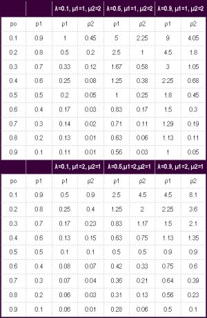
To evaluate performances of calibrated confidence intervals, numerical simulation study was undertaken. Relative coverage is defined as the ratio of coverage percentage to average length of confidence interval. Larger relative coverage implies the better performances of the corresponding confidence intervals. Here we set a continuous distribution with mean 1/λ on inter-arrival time of X₁ and X₂ and a continuous distribution with mean 1/µ₁ on the service time Y₁ at CPU node and that of 1/µ₂ on Y₂ at I/O node. We have considered the values ρ_i <1, i=1, 2 for simulation study from [Table-1] . The intensity parameters ρ_i, i=1, 2 are calculated using [Eq-1] . The different values of λ, µ₁, µ₂, p_o and p₁ are considered as shown in [Table-1] .
For each level of ρ₁ random samples of inter-arrival times and service times (X_1j, p₀Y_1j, j= 1,2...n) are drawn from (X₁, Y₁) respectively. Also for each level of ρ₂ random samples of inter-arrival times and service times (p₁X_2i, p₀Y_2i, j= 1,2...n) are drawn from (X₂, Y₂) respectively. Next N=1000 bootstrap resamples each of size n = 10 and 29 are drawn from the original samples, as well as N=1000 BB replications are simulated for the original samples. According to [Eq-2] to [Eq-9] , we obtain 90% calibrated confidence intervals for intensities ρ_i, i=1, 2. The above simulation process is replicated N=1000 times and we compute coverage percentages, average lengths and relative coverage of the above mentioned calibrated confidence intervals. We utilize a PC Dual Core and apply Matlab®7.0.1 to accomplish all simulations.
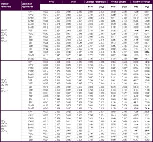
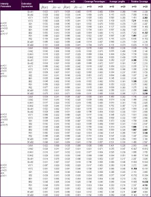
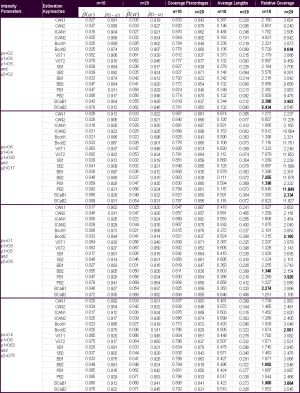
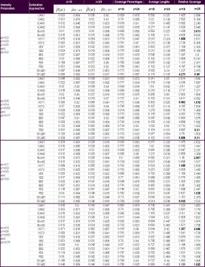
Here C.V. represents coefficient of variation corresponding to the inter-arrival/service time distribution. M represents exponential distribution, E₄ a 4-stage Erlang distribution, $\mathrm{H_{4}^{Pe}}$ a 4-stage hyper-exponential distribution and $\mathrm{H_{4}^{P0}}$ a 4-stage hypo-exponential distribution. Simulated results of $\hat{\beta }(\alpha ),\: \hat{\beta }(1-\alpha )$ , coverage percentage, average lengths and relative coverage for intensities ρ_i, i=1, 2 of a two stage open queueing network models (presented in [Table-2] ) for 90% calibrated confidence intervals with short run are shown in [Table-3] , [Table-4] , [Table-5] , [Table-6] .
According to the simulation results shown in [Table-3] [Table-6] , we find that average lengths are decreasing but both coverage percentages and relative coverage’s are increasing with sample size n. Also we observe that the coverage percentage can approaches to 90% when n increases to 29.
From [Table-7] , we observe that under M/G/1 to G/M/1 model the calibrated confidence intervals with inter-arrival distribution and service time distribution of small CV (<1) have greater relative coverage than those of large CV (>1) for intensities ρ₁ and ρ₂. The estimation approaches Variance-Stabilized Bootstrap-t (VST), Bootstrap-t and Bias-corrected and accelerated bootstrap (BCaB) calibrated confidence interval has the greatest relative coverage. Also the calibrated confidence intervals of model M/E₄/1 to E₄/M/1 shows the greatest relative coverage for ρ₁ and ρ₂. Similarly under G/G/1 to G/G/1 models the calibrated confidence interval with inter-arrival distribution and service time distribution of large CV(>1) have greatest relative coverage than those of small CV(<1) for intensities ρ₁ and ρ₂. The estimation approaches BCaB, VST, PB, Bootstrap-t and BB has the greatest relative coverage. Also the calibrated confidence intervals of model E₄/H₄^Pe/1 to H₄^Pe/E₄/1 show the greatest relative coverage for ρ₁ and ρ₂. Further we observe that average lengths are decreasing and relative coverage increasing with n increases for ρ₁ and ρ₂. It is important to point out that, some poor coverage percentage of above confidence intervals with respect to the nominal level 90% may be due to small sample size n.

Conclusions

This paper provides the calibrated confidence intervals for intensities ρ₁ and ρ₂ of two stage open queueing network with feedback. The relative coverage is adopted to understand, compare and assess performance of the resulted confidence intervals. The simulation results imply that VST, Boot-t and BCaB method has the best performance for M/G/1 to G/M/1 and under G/G/1 to G/G/1 the estimation approach PB, VST, Boot-t, BCaB and BB out performs. The above mentioned approaches are easily applied to practical queueing network such as all types of open, closed, mixed queueing networks as well as cyclic, retrial queueing models.

References

[1] Beran R. (1987) Biometrika, 74, 457-468.
» CrossRef » Google Scholar » PubMed » DOAJ » CAS » Scopus

[2] Burke P.J. (1956) Operations Research, 4, 699-704.
» CrossRef » Google Scholar » PubMed » DOAJ » CAS » Scopus

[3] Disney R.L. (1975) Trans. A.I.E.E., 7, 268-288.
» CrossRef » Google Scholar » PubMed » DOAJ » CAS » Scopus

[4] Efron B. and Gong G. (1983) Am. Stat., 37, 36-48.
» CrossRef » Google Scholar » PubMed » DOAJ » CAS » Scopus

[5] Efron B. and Tibshirani R.J. (1986) Stat. Sci., 1, 54-77.
» CrossRef » Google Scholar » PubMed » DOAJ » CAS » Scopus

[6] Efron B. and Tibshirani R. (1993) An Introduction to the Bootstrap, Chapman and Hall, New York.
» CrossRef » Google Scholar » PubMed » DOAJ » CAS » Scopus

[7] Efron B. (1979) Annals of Statistics, 7, 1-26.
» CrossRef » Google Scholar » PubMed » DOAJ » CAS » Scopus

[8] Efron B. (1982) SIAM Monograph, 38.
» CrossRef » Google Scholar » PubMed » DOAJ » CAS » Scopus

[9] Efron B. (1987) J. Am. Stat. Assoc., 82, 171- 200.
» CrossRef » Google Scholar » PubMed » DOAJ » CAS » Scopus

[10] Guntur B. (1991) Quality Progress, 97-103.
» CrossRef » Google Scholar » PubMed » DOAJ » CAS » Scopus

[11] Hall P. (1986) Ann. Statist., 14, 1431-1452.
» CrossRef » Google Scholar » PubMed » DOAJ » CAS » Scopus

[12] Hall P. and Martin M.A. (1988) Biometrika, 75, 661-671.
» CrossRef » Google Scholar » PubMed » DOAJ » CAS » Scopus

[13] Hogg R.V. and Craig A.T. (1995) Introduction to Mathematical Statistics, Prentice- Hall, Inc.
» CrossRef » Google Scholar » PubMed » DOAJ » CAS » Scopus

[14] Jackson J.R. (1957) Operations Research, 5, 518- 521.
» CrossRef » Google Scholar » PubMed » DOAJ » CAS » Scopus

[15] Ke J.C. and Chu Y.K. (2009) Computational Statistics, 24(4), 567-582.
» CrossRef » Google Scholar » PubMed » DOAJ » CAS » Scopus

[16] Loh W.Y. (1987) J. Amer. Statist. Assoc., 82, 155-162.
» CrossRef » Google Scholar » PubMed » DOAJ » CAS » Scopus

[17] Loh W.Y. (1991) Statistica sinica, 1, 477-491.
» CrossRef » Google Scholar » PubMed » DOAJ » CAS » Scopus

[18] Miller R.G. (1974) Biometrika, 61, 1-15.
» CrossRef » Google Scholar » PubMed » DOAJ » CAS » Scopus

[19] Mooney C.Z. and Duval R.D. (1993) Bootstrapping: a nonparameric approach to Statistical inference, SAGE Newbury Park.
» CrossRef » Google Scholar » PubMed » DOAJ » CAS » Scopus

[20] Rousses G.G. (1997) A Course in Mathematical Statistics, 2nd ed., Academic Press, New York.
» CrossRef » Google Scholar » PubMed » DOAJ » CAS » Scopus

[21] Rubin D.B. (1981) The Annals of Statistics, 9, 130-134.
» CrossRef » Google Scholar » PubMed » DOAJ » CAS » Scopus

[22] Thiruvaiyaru D. and Basava I.V. (1996) Stochastic Processes and Statistical Inference, New Age International Publications, New Delhi, 132-149.
» CrossRef » Google Scholar » PubMed » DOAJ » CAS » Scopus

[23] Thiruvaiyaru D., Basava I.V. and Bhat U.N. (1991) Queueing Systems, 9, 301-312.
» CrossRef » Google Scholar » PubMed » DOAJ » CAS » Scopus

[24] Young G.A. (1994) Stat Sci., 9, 382-415.
» CrossRef » Google Scholar » PubMed » DOAJ » CAS » Scopus

Images

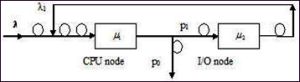	Fig. 1- Two stage open queueing network with feedback
	Table 1- Different levels of intensity parameters considered in the simulation study
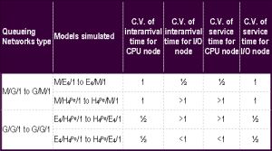	Table 2- Different queueing network models simulated for study
	Table 3- Queueing network model: M/E₄/1 to E₄/M/1.
	Table 4- Queueing network model: M/H₄^Pe/1 to H₄^Pe/M/1.
	Table 5- Queueing network model: E₄/H₄^Pe/1 to H₄^Pe/E₄/1.
	Table 6- Queueing network model: E₄/H₄^Po/1 to H₄^Po/E₄/1. Note [for Table-3 to Table-6] Boldface denotes the greatest relative coverage among estimation approaches. Calibrated confidence intervals of ρ₁ under different estimation approaches are denoted by CAN1, Exact-t1, Boot-t1, VST1, SB1, BB1, PB1, BCaB1 and that of ρ₂ are denoted by CAN2 Exact-t2, Boot-t2, VST2, SB2, BB2, PB2 and BCaB2.
	Table 7- Performances of the estimation approaches of intensities

Licence

ISSN & EISSN

Scan QR Code

Journal Details

Special Issues

Publishing Ethics

Share

CALIBRATED CONFIDENCE INTERVALS FOR INTENSITIES OF A TWO STAGE OPEN QUEUEING NETWORK WITH FEEDBACK

Translate Article

Article Category

Article Statistics

Downloads

Citations

Cited By

Cite

Import Cite

Share

Related Article

Google Scholar

PubMed